Hartmann
Authors: Jonathan Frassineti and Pietro Bonfà
This example reproduces the findings of Hartmann in PRL 39 832 (1977), but in the hard (stupid?!) way, without using the secular approximation and calculating the spread of local magnetic fields directly from the polarization.
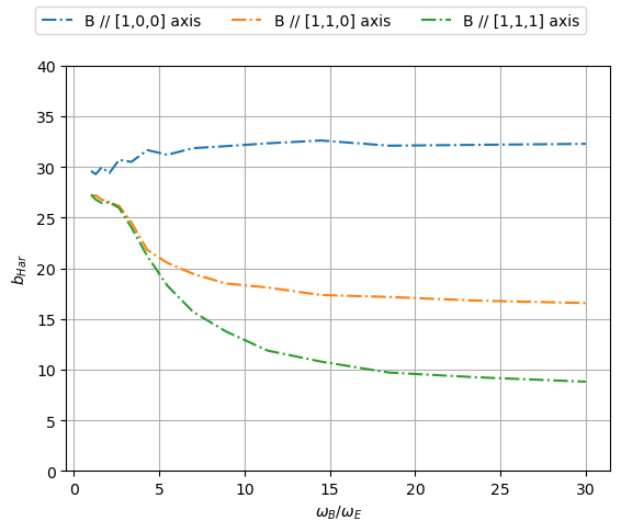
The simulations that follow can for example reproduce the case of Cu for different transverse magnetic fields applied along the [1,0,0], [1,1,0] and [1,1,1] directions.
The different reduced damping rates ‘b_Har’ are shown in the figure. ‘\(b_{Har}\) is related to the width of the Gaussian field distribution \(\Delta_TF\) through the formula:
For a more detailed description see A.Yaouanc and P. de Réotier, Muon Spin Rotation, Relaxation and Resonance, Oxford University Press, 2010, chapter 6, Fig. 6.19 (left).
[1]:
try:
    from undi import MuonNuclearInteraction
except (ImportError, ModuleNotFoundError):
    import sys
    sys.path.append('../undi')
    from undi import MuonNuclearInteraction
import matplotlib.pyplot as plt
import numpy as np
from scipy.optimize import curve_fit
Define physical constants.
[2]:
COMPUTE = False # Computation takes some time (~30 min)
                # When set to False, results previously
                # obtained and stored in this folder are
                # used.

fields = 15 # Number of transversal external fields applied.
angtom = 1.0e-10 # m, Angstrom.
a = 3.6 # Cu lattice constant, in Angstrom.
elementary_charge = 1.6021766e-19 # Elementary charge, in Coulomb = Ampere*second.
epsilon0 = 8.8541878e-12 # Vacuum permittivity, in Ampere^2*kilogram^−1*meter^−3*second^4.
mu0 = 4*np.pi*1e-7 # Hm^-1
h = 6.6260693e-34 # J*s, Planck's constant.
hbar = h/(2*np.pi) # J*s, reduced Planck's constant.

gamma_mu = 2*np.pi*135.5e6 # sT^-1, gyromagnetic ratio of muon.
gamma_Cu = 71.118e6 # sT^-1, gyromagnetic ratio of Cu.
omega = -1.378879e6/3. # Quadrupolar resonance frequency of Cu, in s^-1.

def rotation_matrix(axis, theta):
    """
    Return the rotation matrix associated with counterclockwise rotation about
    the given axis by theta radians.
    https://stackoverflow.com/a/6802723
    """
    axis = np.asarray(axis)
    axis = axis / np.sqrt(np.dot(axis, axis))
    a = np.cos(theta / 2.0)
    b, c, d = -axis * np.sin(theta / 2.0)
    aa, bb, cc, dd = a * a, b * b, c * c, d * d
    bc, ad, ac, ab, bd, cd = b * c, a * d, a * c, a * b, b * d, c * d
    return np.array([[aa + bb - cc - dd, 2 * (bc + ad), 2 * (bd - ac)],
                     [2 * (bc - ad), aa + cc - bb - dd, 2 * (cd + ab)],
                     [2 * (bd + ac), 2 * (cd - ab), aa + dd - bb - cc]])
Define the atomic positions for muon and Cu nuclei. We also rotate the corresponding atomic positions (and so the axis) in order to have the external fields along x, and the muon spin along z.
These are the original positions.
[3]:
pos = np.array ([[0., 0., 0.5],
                 [0. ,  0.,  0.],
                 [0. ,  0.,  1.],
                 [0.5 ,  0.,  0.5],
                 [-0.5 ,  0.,  0.5],
                 [0. ,  0.5,  0.5],
                 [0. ,  - 0.5,  0.5]])*angtom*a
Define the atomic structure.
[4]:
def gen_atoms(positions):
    """
    This function returns the input for UNDI assuming that the muon
    is the first position.
    """
    return [
                {'Position': positions[i],
                    'Label': 'mu'
                } if i == 0 else # first element is the muon

                {'Position': positions[i],
                    'Label': '63Cu',
                    'OmegaQmu': 3*omega
                } for i in range(7) # 6 atoms + 1 muon
            ]
Polarization function.
The muon polarization is obtained with the method introduced by celio_on_steroids.
[5]:
time_max = 20e-6 # Value of the temporal window, in seconds.
freq_max = 400e6 # Value of the sampling frequency, in Hz.
                 # This is 10 times the maximum Larmor frequency used in this sample,
                 # about 40 MHz. This has been done to avoid aliasing.

steps = int(freq_max*time_max) # Number of steps used to simulate the signal.
tlist = np.linspace(0,time_max,steps) # Time scale, in seconds.
Define the applied external transverse magnetic fields, in Tesla. With these values, we obtain a maximum applied external field of 0.58 T.
[6]:
factors = np.logspace(np.log2(1),np.log2(30),fields,base=2)
TF = factors * np.abs(omega)/gamma_Cu
# direction of transverse field
B_dir = np.array([1.,0.,0.])

# Computation is long and when COMPUTE==False stored values are used.
if COMPUTE:
    print("Computing signal for positive EFGs...", end='', flush=True)

    signal = np.zeros((fields, 3, steps))

    for i in range(fields):
        #| Align the magnetic fields along x.
        B = TF[i]*B_dir

        # do not rotate aanything yet
        R = np.eye(3)
        rpos = np.dot(R,pos.T).T
        NS = MuonNuclearInteraction(gen_atoms(rpos), external_field=B, log_level='info')
        signal[i,0,:] = NS.celio_on_steroids(tlist,  k=1) + NS.celio_on_steroids(tlist,  k=1)
        del NS

        # rotate 45 deg with axis=z to get [110] along B direction, which is x
        R = rotation_matrix([0,0,1], np.pi/4)
        rpos = np.dot(R,rpos.T).T
        NS = MuonNuclearInteraction(gen_atoms(rpos), external_field=B, log_level='info')
        signal[i,1,:] = NS.celio_on_steroids(tlist,  k=1) + NS.celio_on_steroids(tlist,  k=1)
        del NS

        # rotate 45 deg again, but this time with axis y.
        R = rotation_matrix([0,1,0], np.pi/4)
        rpos = np.dot(R,rpos.T).T
        NS = MuonNuclearInteraction(gen_atoms(rpos), external_field=B, log_level='info')
        signal[i,2,:] = NS.celio_on_steroids(tlist,  k=1) + NS.celio_on_steroids(tlist,  k=1)
        del NS

    signal /= 2.
    print('done!')
else:
    data = np.load('Hartmann.npz')
    tlist = data.get('tlist')
    signal = data.get('signal')
Real space analysis
In a μSR-experiment data are collected from a large number of decaying muons, each sitting in a different field determined by the local arrangement of its surrounding nuclear moments. The distribution of these local fields is Gaussian, with average value zero and the width determined by the spread \(\langle \DeltaB^2 _{dip}\rangle\). If an external field \(B_{ext}\) is applied, the average precession frequency of the muon system will still be ωB = (gμμN/ℏ)Bext, but the distribution of the fields will give rise to a damping factor of the of the form exp(−σ2t2) with σ = (1/√2)(gμμN/ℏ)√⟨ΔB2dip⟩. This form of damping is called Gaussian. The magnitude of the damping factor σ depends on the spins of the nuclei (I), the strength of the nuclear dipoles μI = gIIμN and on the position (distance ri and angle θi with respect to the applied magnetic field Bext) of the surrounding nuclei
[7]:
bhar = np.empty((fields, 3))

def damped_oscillation(x, *p):
    gB, sigma = p
    return np.cos(gB*x)*np.exp(-0.5*(sigma*x)**2)

for i in range(fields):
    for j in range(3):

        coeff, var_matrix = curve_fit(damped_oscillation, tlist,
                                      signal[i,j],
                                      p0=[gamma_mu*TF[i], 1e6]
                                      )
        gammaB, sigma = np.abs(coeff)
        # We calculate the width of the field distribution 'delta_TF' at
        # the muon site.
        Delta_TF = sigma/gamma_mu
        # Finally, we calculate the reduced damping rate 'b_Har' for the
        # three different magnetic field orientations.
        bhar[i,j] = (4*np.pi*Delta_TF*(a*angtom)**3)/(gamma_Cu*hbar*mu0)

fig, axes = plt.subplots(1, 1)
axes.plot(factors,bhar[:,0], label = 'B // [1,0,0] axis', linestyle='-.')
axes.plot(factors,bhar[:,1], label = 'B // [1,1,0] axis', linestyle='-.')
axes.plot(factors,bhar[:,2], label = 'B // [1,1,1] axis', linestyle='-.')
axes.set_ylabel('$b_{Har}$')
axes.set_xlabel('$\omega_B/\omega_E$')
axes.set_ylim([0,40])
axes.grid()
fig.legend(loc=9,ncol=3)
plt.show()
<>:27: SyntaxWarning: "\o" is an invalid escape sequence. Such sequences will not work in the future. Did you mean "\\o"? A raw string is also an option.
<>:27: SyntaxWarning: "\o" is an invalid escape sequence. Such sequences will not work in the future. Did you mean "\\o"? A raw string is also an option.
/tmp/ipykernel_548098/1165114285.py:27: SyntaxWarning: "\o" is an invalid escape sequence. Such sequences will not work in the future. Did you mean "\\o"? A raw string is also an option.
  axes.set_xlabel('$\omega_B/\omega_E$')
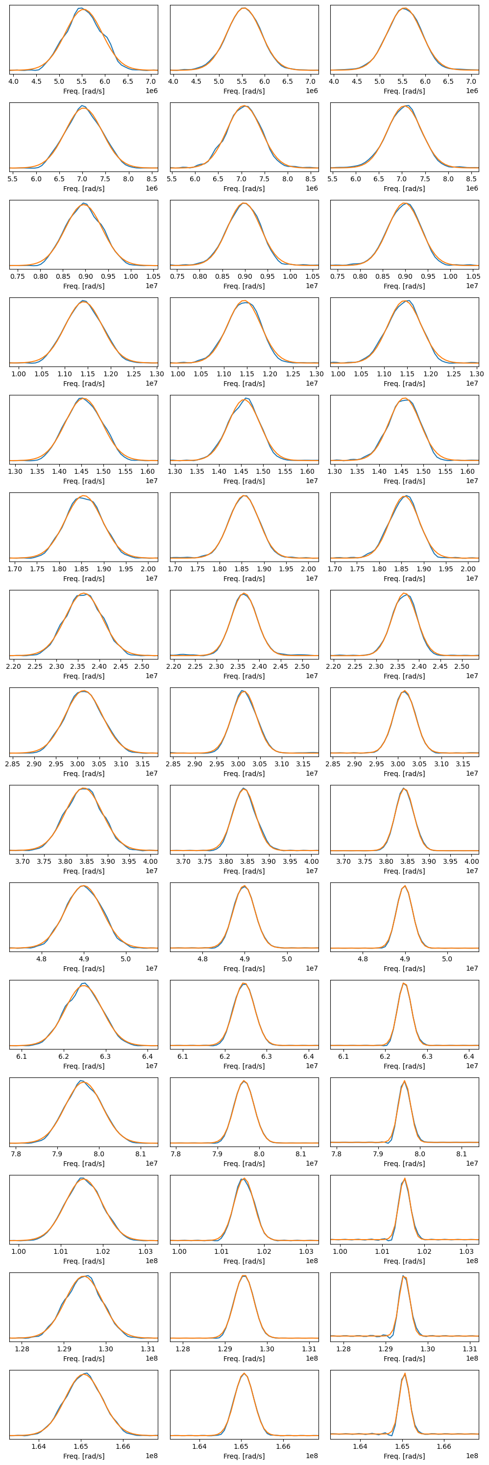
Fourier transform
That same can be obtained from the Fourier transform of the simulated polarization functions. The polarization function for a transverse filed is approximated by:
The Fourier Transform of this signal is
Assuming the field distribution to be Gaussian, the width (\(\sigma\)) can be obtained from the (real part of the) Fourier transform.
[8]:
# Add some interpolation
zero_padding = 4
# prepare spaze for Fourier transforms...
yf = np.empty((fields, 3, zero_padding*len(tlist)//2+1), dtype=complex)
# ...but work in omega domain, not in frequency, notice   VVV
xf = np.fft.rfftfreq(zero_padding*len(tlist), tlist[1]/(2*np.pi))

amp      = np.empty((fields, 3))
mean     = np.empty((fields, 3))
stddev   = np.empty((fields, 3))
bhar     = np.empty((fields, 3))
Fourier transform of i-th polarization signal for the three axis.
[9]:
def gauss(x, *p):
    A, mu, sigma = p
    return A*np.exp(-0.5*(x-mu)**2/(sigma**2))

for i in range(fields):
    for j in range(3):
        yf[i,j] = np.fft.rfft(signal[i,j], zero_padding*len(tlist))
        # Gaussian fit of the real part of the FFT.
        coeff, var_matrix = curve_fit(gauss, xf,
                                      np.real(yf[i,j]),
                                      p0=[np.real(yf[i,j]).max(),
                                          xf[np.argmax(np.real(yf[i,j]))],
                                          200000]
                                      )
        amp[i,j], mean[i,j], stddev[i, j] = np.abs(coeff)
        # We calculate the width of the field distribution 'delta_TF' at
        # the muon site.
        Delta_TF = stddev[i, j]/gamma_mu
        # Finally, we calculate the reduced damping rate 'b_Har' for the
        # three different magnetic field orientations.
        bhar[i,j] = (4*np.pi*Delta_TF*(a*angtom)**3)/(gamma_Cu*hbar*mu0)
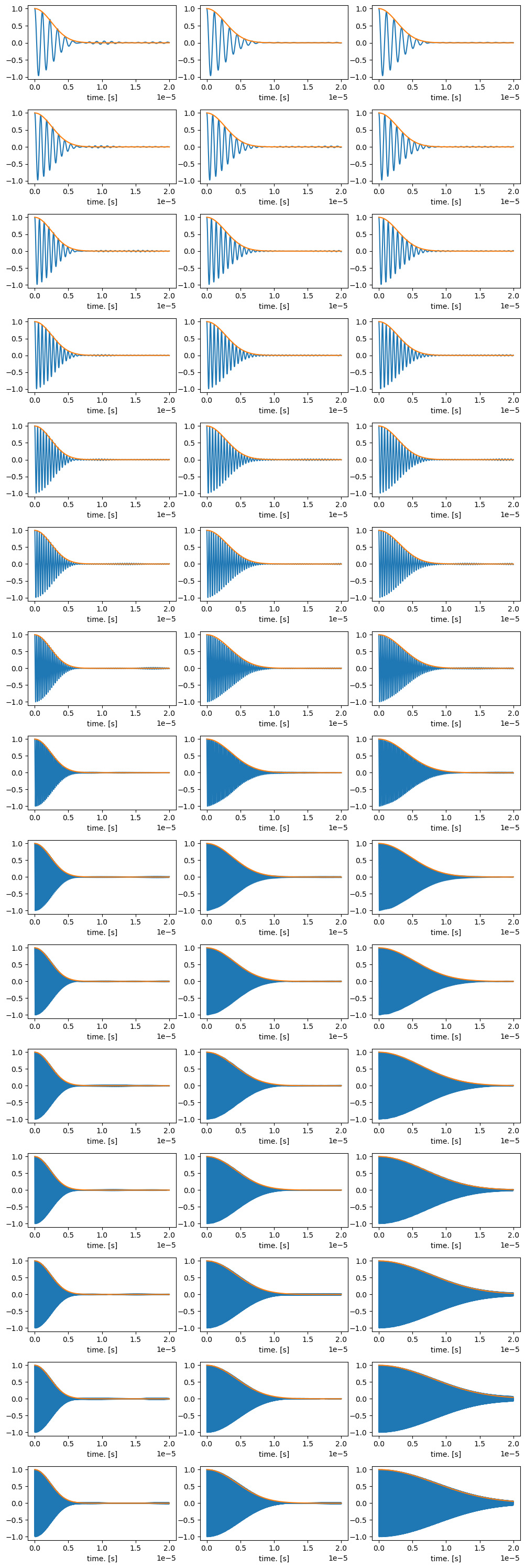
Plot time functions
[10]:
ncols = 3
nrows = fields
fig, axes = plt.subplots(nrows, ncols, figsize=(10,30))
l=0
for ax in axes.flat:
    i=l//3
    j=l%3
    ax.plot(tlist,signal[i,j])
    ax.plot(tlist,np.exp(-0.5*(stddev[i, j]**2)*tlist**2))
    ax.set_xlabel('time. [s]')
    l += 1
fig.tight_layout()
plt.show()
Plot the Fourier transforms.
[11]:
ncols = 3
nrows = fields
fig, axes = plt.subplots(nrows, ncols, figsize=(10,30))
l=0
for ax in axes.flat:
    i=l//3
    j=l%3
    ax.plot(xf,yf[i,j].real)
    ax.plot(xf,gauss(xf,amp[i,j], mean[i,j], stddev[i, j]))
    ax.set_xlim([mean[i,j]-4*np.max(stddev[i, :]),mean[i,j]+4*np.max(stddev[i, :])])
    ax.set(yticks=[])
    ax.set_xlabel('Freq. [rad/s]')
    l += 1
fig.tight_layout()
plt.show()
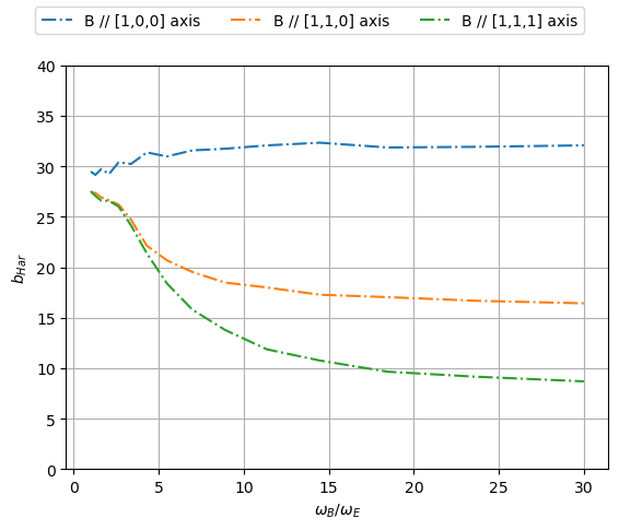
Eventually plot \(b_{Har}\) that compares directly with the results available in the letter cited at the beginning of this example.
[12]:
fig, axes = plt.subplots(1, 1)
axes.plot(factors,bhar[:,0], label = 'B // [1,0,0] axis', linestyle='-.')
axes.plot(factors,bhar[:,1], label = 'B // [1,1,0] axis', linestyle='-.')
axes.plot(factors,bhar[:,2], label = 'B // [1,1,1] axis', linestyle='-.')
axes.set_ylabel('$b_{Har}$')
axes.set_xlabel('$\omega_B/\omega_E$')
axes.set_ylim([0,40])
axes.grid()
fig.legend(loc=9,ncol=3)
plt.show()
<>:6: SyntaxWarning: "\o" is an invalid escape sequence. Such sequences will not work in the future. Did you mean "\\o"? A raw string is also an option.
<>:6: SyntaxWarning: "\o" is an invalid escape sequence. Such sequences will not work in the future. Did you mean "\\o"? A raw string is also an option.
/tmp/ipykernel_548098/652547007.py:6: SyntaxWarning: "\o" is an invalid escape sequence. Such sequences will not work in the future. Did you mean "\\o"? A raw string is also an option.
  axes.set_xlabel('$\omega_B/\omega_E$')